Experiment 8 - Mixer

Michael Smith
ELEC 3030-RF Systems Lab
Date of Lab - Friday, October 28, 2021, 1 p.m.
Experiment 8 – Mixer
Today’s Date - December 2, 2021
Introduction
The mixer multiplies an RF signal with an oscillator signal to produce a number of signals at different frequencies. The desired output is known as the difference frequency, which in our radio is termed the intermediate frequency, or If. This lab is designed to help us become familiar with how a mixer works. To help us do so, we have to analyze the mixer in LTspice, generating spectrums using the FFT function. All of this is done to help us be well educated and prepared to breadboard various mixer circuits and test them during our lab.
In order to cut on redundancy and reduce the addition of unnecessary images, I have labeled my images the same as the images in the lab instructions. In other words, if the lab instructions say to recreate the circuit in Figure 8.4, I have labeled the circuit I recreated from the lab instructions, Figure 8.4. Likewise, if we are to recreate Table 8.3, I have labeled my Table 8.3, same with graphs. Since the person grading this paper is very familiar with the pre-lab and lab instructions, I don’t see the need to add the images that have to be recreated when the reader has that information in front of them. Also, I feel if you must compare lab instructions of Figure 8.3 to my Figure 8.3, it cuts down on confusion of numbering and labeling.
Part 8.3 Step 1-3
In the first part of this lab, we had to physically build the circuit as in the diagram of Figure 8.3, which is the default mixer circuit. Then on our oscilloscope we had to observe the output across the load. We had to inspect the output spectrum as we varied the oscillator frequency, see Figures 1 and 2. From these figures there are very noticeable spikes. These spikes are the RF signal and the local oscillator (LO) signal. The frequency we need to observe is the intermediate frequency. In our case the intermediate frequency is located at 200kHz. The mixer circuit gives us the ability to modify the frequency of the input RF signal from 1MHz to 200kHz. This frequency is much easier to filter through a Band-Pass filter.
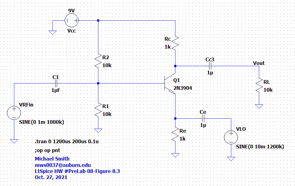

Figure 8.3 – Default Mixing Circuit
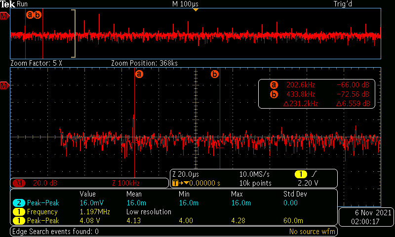
Figure 1 - 200 KHz Intermediate Frequency (IF)
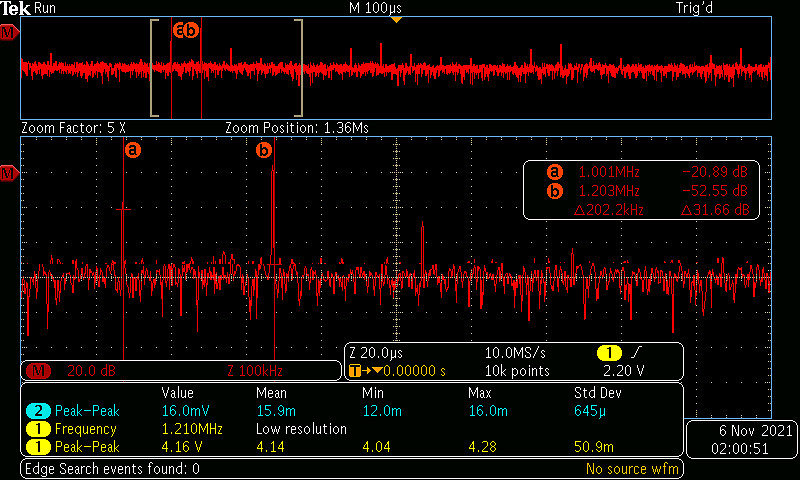
Figure 2 - RF 1MHz and Local Oscillator (LO) 1.2MHz signals.
Part 8.3 Step 4
In this part of our lab experiment we repeated the same steps of 1-3. This time though, in our circuit we added an RFC, see Figure 8.5 below. The output spectrum took measurements over our new circuit, see Figures 3 and 4, again from these figures there are very noticeable spikes. Comparing Figures 3 and 4 to Figures 1 and 2 the intermediate frequency of 200kHz is much larger than in Figures 1 and 2. This means this mixer circuit will have better performance and have less of a loss.
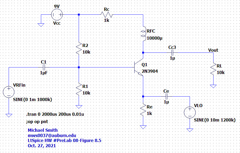
Figure 8.5 – Mixer circuit with an RFC added
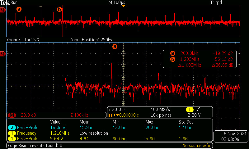
Figure 3 - 200 KHz Intermediate Frequency (IF)
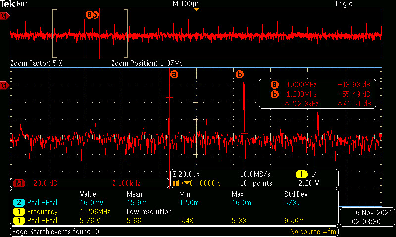
Figure 4 – RF 1MHz and Local Oscillator (LO) 1.2MHz signals.
Part 8.3 Step 5
In the final step of this lab, we needed to add the bandpass filter to complete the circuit in Figure 8.6. We had to complete steps 1-3 on this new circuit, as well. In our lab instructions we were cautioned that our components were not ideal and may have inaccuracies. We were guided to change the LO signal frequency until we observed our largest spike in IF, the resulting oscilloscope image is in Figure 5. From Figure 5 you can see the LO frequency is 1.218 MHz, this means our IF is 218kHz. This is different from 200kHz that was measured from our previous circuits without the filter attached.
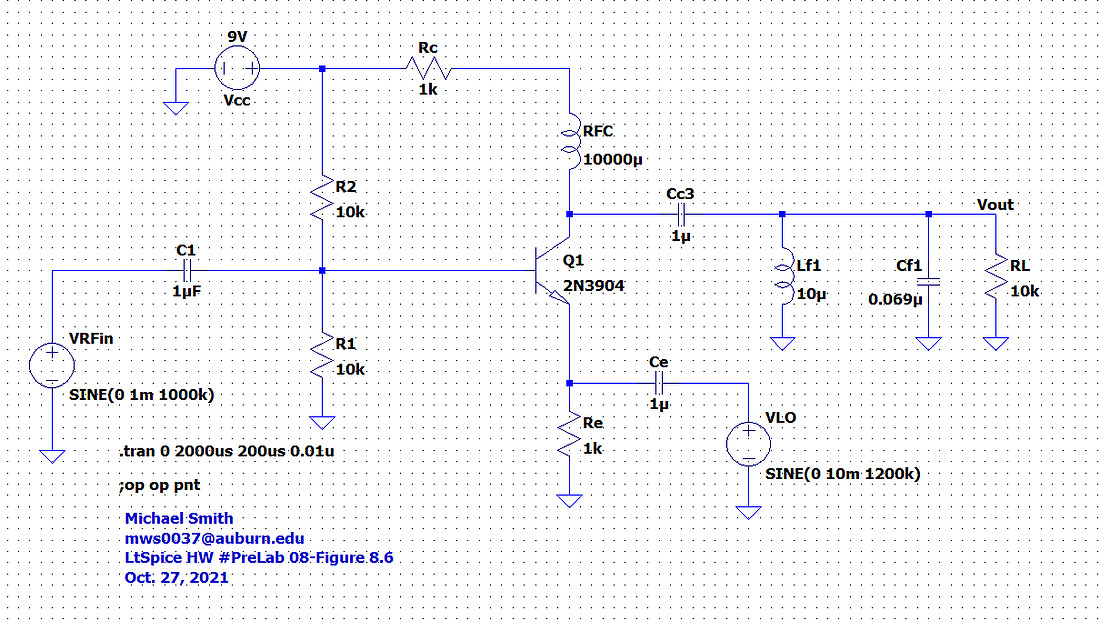
Figure 8.6 – Mixer Circuit with RFC and BPF added
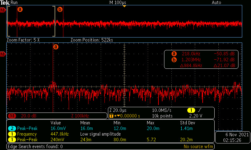
Figure 5 – 218 KHz Intermediate Frequency (IF)
Conclusion
The prelab exercises helped us understand how the mixer multiplies an RF signal with an oscillator signal to produce a number of signals at different frequencies. Analyzing the different mixers in LTspice and generating spectrums using the FFT function helped me see how the addition of capacitors, inductors and even changing RE would affect the gain of my circuit. This has helped me be better prepared to breadboard different mixer circuits and test them in lab. All of these steps are getting us closer to complete the construction of a heterodyne radio. This type of radio will have the ability to shift the incoming high-frequency signal to a lower signal that will have a better performance in filtering and amplification. Adding the Band Pass Filter (BPF) in the final step of this lab eliminated the spikes at 1MHz and 1.218 MHz. After completing this final step, we can now control the signal reaching our radio.